The Housing Market Puzzle: Understanding Local Trends and Pricing Challenges

Real estate economics is far from the trendiest area in economics. At first glance, this seems odd since real estate economics is very complex. It is a truism in economics that the more complex a good, the harder it is for the market to price that good. A common example given is the labor market. After all, there is nothing bought and sold that is more complex than a person’s time. I do not claim that houses are as complex as workers but this does not mean that the housing market is simpler than the labor market. There are a few reasons why this is so. 

Firstly, the labor market and the housing market are closely related. Even after the pandemic, there remains a strong relationship between where people live and where they work. The fact that this relationship has weakened actually makes it more challenging to understand a given housing market. The first point leads into the second. The housing market is inevitably local. Globalization patterns notwithstanding, there is at least one market that must remain local as a house exists in a particular place. 

If this were all, we housing economists would still have our work cut out for us but there is more. When I go to the store to buy milk, I am the buyer and the store is the seller. The supply and demand analysis taught in basic economics courses is easily applied to this situation. In real estate, by contrast, the buyer is often also a seller; that is, many participants in the housing market are on both sides of the transaction. Why does this complicate the picture? 

I can determine my budget for milk knowing only the price of milk. If I am a homeowner who is also a home buyer, my budget for my next house is heavily influenced by the sale price of my current house. This is not something I am necessarily certain of when I begin looking. This is true whether I am looking in the same area or looking to move. This means that the would-be home owner-buyer is at the mercy of economic trends in at least one locality and often two. 

Alas, this is not all. Renting is a substitute for owning and thus the housing market is affected by the rental market. Finally, only a minority of participants in the housing market can buy a home in cash. This means that a home buyer’s budget is also affected by interest rates, that is the price of credit. 

Any seller of a home naturally wishes to sell at the highest price that clears the market. Often, sellers need guidance from realtors on what that price might be. This price changes over time. Firstly, when one examines trends in sales volume and price over time, the trends display what statisticians call seasonality. The easiest way to understand seasonality is to think of temperature. Winter is colder than summer with spring and autumn coming in between. Plotting average temperature month to month over time shows clear cycles. Many such “time series”, as statisticians call data plotted over time, display seasonality. Home prices and sales volume are no exception. However, there is still more to say about the housing market. Recall that I discussed the necessary locality of the housing market. While all housing markets will display seasonality and trends over time, there is still more interesting variation. 

This has all been very abstract so it is time to discuss some concrete data. Let us examine some counties. 

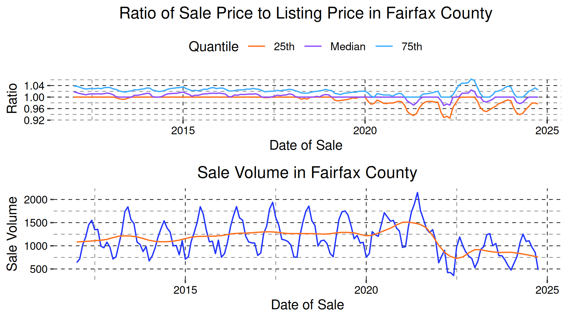
The top plot is the ratio of the listing price to the sale price in Fairfax County VA. Now, when a home sells exactly for its listing price, the ratio of the sale price to the listing price is 1. I have plotted the quantiles of this ratio over time in Fairfax County. To review, the 75th quantile ratio refers to that ratio below which three-quarters of the data fall. The median, or 50th percentile is that value which splits the data in half. The top graph shows that the ratios have remained relatively close to 1, meaning that most homes sell very close to their listing price. That the median is above 1 means that often sellers try to sell for a higher price than clears the market which makes intuitive sense. 

The bottom graph shows the sales volume in Fairfax County over the same time frame. The blue line is the actual sales volume which shows clear seasonality. The red line is the same time series with the seasonality removed. This allows us to better understand long-term trends. Notice that when sales volume rose and then fell, as happened due first to the pandemic and then to the interest rate hikes, the 25th and 75th percentile ratios shifted further from the medians. The point is that when interest rates rose and sales volumes fell, market uncertainty increased and realtors and sellers had more difficulty pricing homes to sell. Naturally, there is some regional variation.

Now let us examine the same plot for Fulton County, GA. 

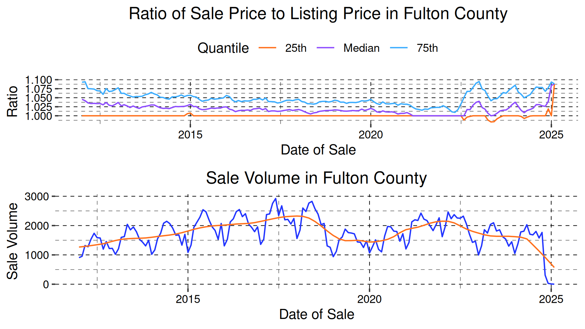
The trend is similar but notice that the 25th percentile ratio is flat at 1 until very recently. Unlike Maricopa, home sellers seem mostly surprised in the upward direction; in other words, many sellers sell for more than their asking price. Here, the spread seems more uniform after 2020.

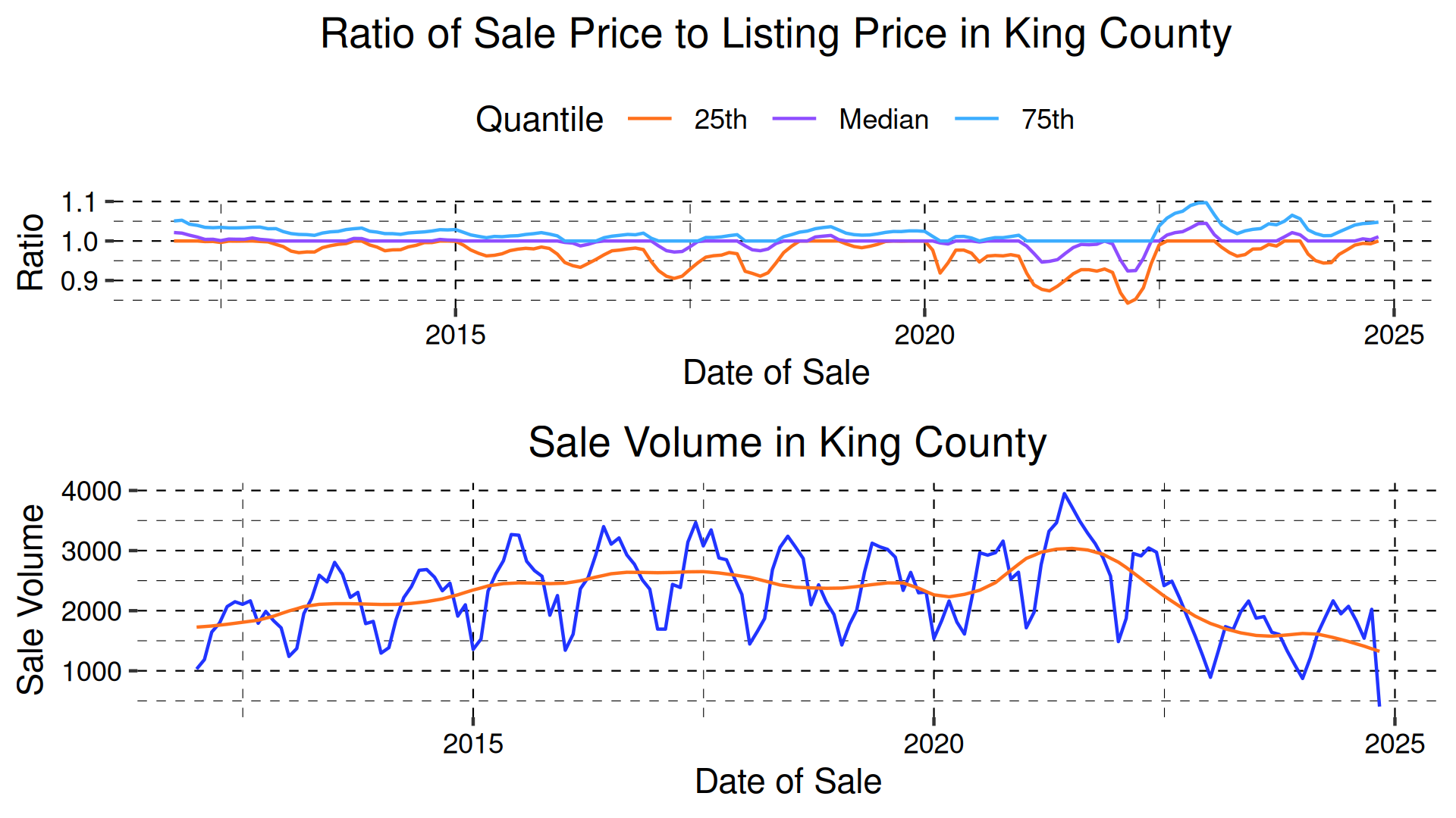
King County, WA shows yet another trend. Again, market uncertainty shoots up when volume falls but here it is the 75th percentile ratio that trends close to 1 over time. This perhaps suggests some over-optimism among King County homeowners. 

Last but not least, consider Maricopa County, AZ.

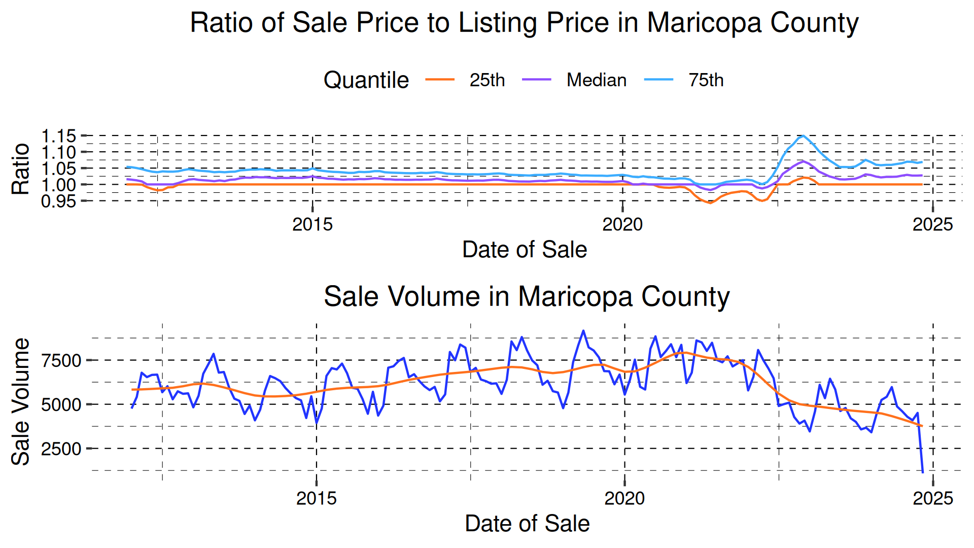
As was the case with Fairfax, the later spread is larger. 

It will take years for real estate economists to understand these trends as much relevant data is not yet available. Nonetheless, a consistent lesson across varied geography is that market uncertainty has increased and thus listing a home at the market clearing price has become more difficult. This is an environment in which analytical sophistication in one’s approach to real estate becomes more valuable.

John Schuler

John Schuler is a Senior Economist at Kukun with expertise in economics, statistics, and agent-based modeling. His research interests include real estate economics and banking. John holds a Ph.D. in Economics from George Mason University and a M.S. in Statistics from American University.

Published November 14, 2024